When something goes wrong, we often strive to be better prepared if the same thing happens again. But the same disasters tend not to happen twice in a row. A more effective approach is simply to prepare to be surprised by life, instead of expecting the past to repeat itself.

***

If we want to become less fragile, we need to stop preparing for the last disaster.

When disaster strikes, we learn a lot about ourselves. We learn whether we are resilient, whether we can adapt to challenges and come out stronger. We learn what has meaning for us, we discover core values, and we identify what we’re willing to fight for. Disaster, if it doesn’t kill us, can make us stronger. Maybe we discover abilities we didn’t know we had. Maybe we adapt to a new normal with more confidence. And often we make changes so we will be better prepared in the future.

But better prepared for what?

After a particularly trying event, most people prepare for a repeat of whatever challenge they just faced. From the micro level to the macro level, we succumb to the availability bias and get ready to fight a war we’ve already fought. We learn that one lesson, but we don’t generalize that knowledge or expand it to other areas. Nor do we necessarily let the fact that a disaster happened teach us that disasters do, as a rule, tend to happen. Because we focus on the particulars, we don’t extrapolate what we learn to identifying what we can better do to prepare for adversity in general.

We tend to have the same reaction to challenge, regardless of the scale of impact on our lives.

Sometimes the impact is strictly personal. For example, our partner cheats on us, so we vow never to have that happen again and make changes designed to catch the next cheater before they get a chance; in future relationships, we let jealousy cloud everything.

But other times, the consequences are far reaching and impact the social, cultural, and national narratives we are a part of. Like when a terrorist uses an airplane to attack our city, so we immediately increase security at airports so that planes can never be used again to do so much damage and kill so many people.

The changes we make may keep us safe from a repeat of those scenarios that hurt us. The problem is, we’re still fragile. We haven’t done anything to increase our resilience—which means the next disaster is likely to knock us on our ass.

Why do we keep preparing for the last disaster?

Disasters cause pain. Whether it’s emotional or physical, the hurt causes vivid and strong reactions. We remember pain, and we want to avoid it in the future through whatever means possible. The availability of memories of our recent pain informs what we think we should do to stop it from happening again.

This process, called the availability bias, has significant implications for how we react in the aftermath of disaster. Writing in The Legal Analyst: A Toolkit for Thinking about the Law about the information cascades this logical fallacy sets off, Ward Farnsworth says they “also help explain why it’s politically so hard to take strong measures against disasters before they have happened at least once. Until they occur they aren’t available enough to the public imagination to seem important; after they occur their availability cascades and there is an exaggerated rush to prevent the identical thing from happening again. Thus after the terrorist attacks on the World Trade Center, cutlery was banned from airplanes and invasive security measures were imposed at airports. There wasn’t the political will to take drastic measures against the possibility of nuclear or other terrorist attacks of a type that hadn’t yet happened and so weren’t very available.”

In the aftermath of a disaster, we want to be reassured of future safety. We lived through it, and we don’t want to do so again. By focusing on the particulars of a single event, however, we miss identifying the changes that will improve our chances of better outcomes next time. Yes, we don’t want any more planes to fly into buildings. But preparing for the last disaster leaves us just as underprepared for the next one.

What might we do instead?

We rarely take a step back and go beyond the pain to look at what made us so vulnerable to it in the first place. However, that’s exactly where we need to start if we really want to better prepare ourselves for future disaster. Because really, what most of us want is to not be taken by surprise again, caught unprepared and vulnerable.

The reality is that the same disaster is unlikely to happen twice. Your next lover is unlikely to hurt you in the same way your former one did, just as the next terrorist is unlikely to attack in the same way as their predecessor. If we want to make ourselves less fragile in the face of great challenge, the first step is to accept that you are never going to know what the next disaster will be. Then ask yourself: How can I prepare anyway? What changes can I make to better face the unknown?

As Andrew Zolli and Ann Marie Healy explain in Resilience: Why Things Bounce Back, “surprises are by definition inevitable and unforeseeable, but seeking out their potential sources is the first step toward adopting the open, ready stance on which resilient responses depend.”

Giving serious thought to the range of possible disasters immediately makes you aware that you can’t prepare for all of them. But what are the common threads? What safeguards can you put in place that will be useful in a variety of situations? A good place to start is increasing your adaptability. The easier you can adapt to change, the more flexibility you have. More flexibility means having more options to deal with, mitigate, and even capitalize on disaster.

Another important mental tool is to accept that disasters will happen. Expect them. It’s not about walking around every day with your adrenaline pumped in anticipation; it’s about making plans assuming that they will get derailed at some point. So you insert backup systems. You create a cushion, moving away from razor-thin margins. You give yourself the optionality to respond differently when the next disaster hits.

Finally, we can find ways to benefit from disaster. Author and economist Keisha Blair, in Holistic Wealth, suggests that “building our resilience muscles starts with the way we process the negative events in our lives. Mental toughness is a prerequisite for personal growth and success.” She further writes, “adversity allows us to become better rounded, richer in experience, and to strengthen our inner resources.” We can learn from the last disaster how to grow and leverage our experiences to better prepare for the next one.

The post Stop Preparing For The Last Disaster appeared first on Farnam Street.

Posted by Ehsan Amid, Student Researcher and Rohan Anil, Software Engineer, Google Research

The quality of models produced by machine learning (ML) algorithms directly depends on the quality of the training data, but real world datasets typically contain some amount of noise that introduces challenges for ML models. Noise in the dataset can take several forms from corrupted examples (e.g., lens flare in an image of a cat) to mislabelled examples from when the data was collected (e.g., an image of cat mislabelled as a flerken).

The ability of an ML model to deal with noisy training data depends in great part on the loss function used in the training process. For classification tasks, the standard loss function used for training is the logistic loss. However, this particular loss function falls short when handling noisy training examples due to two unfortunate properties:

1. Outliers far away can dominate the overall loss: The logistic loss function is sensitive to outliers. This is because the loss function value grows without bound as the mislabelled examples (outliers) are far away from the decision boundary. Thus, a single bad example that is located far away from the decision boundary can penalize the training process to the extent that the final trained model learns to compensate for it by stretching the decision boundary and potentially sacrificing the remaining good examples. This “large-margin” noise issue is illustrated in the left panel of the figure below.
2. Mislabeled examples nearby can stretch the decision boundary: The output of the neural network is a vector of activation values, which reflects the margin between the example and the decision boundary for each class. The softmax transfer function is used to convert the activation values into probabilities that an example will belong to each class. As the tail of this transfer function for the logistic loss decays exponentially fast, the training process will tend to stretch the boundary closer to a mislabeled example in order to compensate for its small margin. Consequently, the generalization performance of the network will immediately deteriorate, even with a low level of label noise (right panel below).

We visualize the decision surface of a 2-layered neural network as it is trained for binary classification. Blue and orange dots represent the examples from the two classes. The network is trained with logistic loss under two types of noisy conditions: (left) large-margin noise and (right) small-margin-noise.

We tackle these two problems in a recent paper by introducing a “bi-tempered” generalization of the logistic loss endowed with two tunable parameters that handle those situations well, which we call “temperatures”—t₁, which characterizes boundedness, and t₂ for tail-heaviness (i.e. the rate of decline in the tail of the transfer function). These properties are illustrated below. Setting both t₁ and t₂ to 1.0 recovers the logistic loss function. Setting t₁ lower than 1.0 increases the boundedness and setting t₂ greater than 1.0 makes for a heavier-tailed transfer function. We also introduce this interactive visualization which allows you to visualize the neural network training process with the bi-tempered logistic loss.

Left: Boundedness of the loss function. When t1 is between 0 and 1, exclusive, only a finite amount of loss is incurred for each example, even if they are mislabeled. Shown is t1 = 0.8. Right: Tail-heaviness of the transfer function. The heavy-tailed transfer function applies when t2 = > 1.0 and assigns higher probability for the same amount of activation, thus preventing the boundary from drawing closer to the noisy example. Shown is t2 = 2.0.

To demonstrate the effect of each temperature, we train a two-layer feed-forward neural network for a binary classification problem on a synthetic dataset that contains a circle of points from the first class, and a concentric ring of points from the second class. You can try this yourself on your browser with our interactive visualization. We use the standard logistic loss function, which can be recovered by setting both temperatures equal to 1.0, as well as our bi-tempered logistic loss for training the network. We then demonstrate the effects of each loss function for a clean dataset, a dataset with small-margin noise, large-margin noise, and a dataset with random noise.

Logistic vs. bi-tempered logistic loss: (a) noise-free labels, (b) small-margin label noise, (c) large-margin label noise, and (d) random label noise. The temperature values (t1, t2) for the tempered loss are shown above each figure. We find that for each situation, the decision boundary recovered by training with the bi-tempered logistic loss function is better than before.

Noise Free Case:
We show the results of training the model on the noise-free dataset in column (a), using the logistic loss (top) and the bi-tempered logistic loss (bottom). The white line shows the decision boundary for each model. The values of (t₁, t₂), the temperatures in the bi-tempered loss function, are shown below each column of the figure. Notice that for this choice of temperatures, the loss is bounded and the transfer function is tail-heavy. As can be seen, both losses produce good decision boundaries that successfully separates the two classes.

Small-Margin Noise:
To illustrate the effect of tail-heaviness of the probabilities, we artificially corrupt a random subset of the examples that are near the decision boundary, that is, we flip the labels of these points to the opposite class. The results of training the networks on data with small-margin noise using the logistic loss as well as the bi-tempered loss is shown in column (b).

As can be seen, the logistic loss, due to the lightness of the softmax tail, stretches the boundary closer to the noisy points to compensate for their low probabilities. On the other hand, the bi-tempered loss using only the tail-heavy probability transfer function by adjusting t₂ can successfully avoid the noisy examples. This can be explained by the heavier tail of the tempered exponential function, which assigns reasonably high probability values (and thus, keeps the loss value small) while maintaining the decision boundary away from the noisy examples.

Large-Margin Noise:
Next, we evaluate the performance of the two loss functions for handling large-margin noisy examples. In (c), we randomly corrupt a subset of the examples that are located far away from the decision boundary, the outer side of the ring as well as points near the center).

For this case, we only use the boundedness property of the bi-tempered loss, while keeping the softmax probabilities the same as the logistic loss. The unboundedness of the logistic loss causes the decision boundary to expand towards the noisy points to reduce their loss values. On the other hand, the bounded bi-tempered loss, bounded by adjusting t₁, incurs a finite amount of loss for each noisy example. As a result, the bi-tempered loss can avoid these noisy examples and maintain a good decision boundary.

Random Noise:
Finally, we investigate the effect of random noise in the training data on the two loss functions. Note that random noise comprises both small-margin and large-margin noisy examples. Thus, we use both boundedness and tail-heaviness properties of the bi-tempered loss function by setting the temperatures to (t₁, t₂) = (0.2, 4.0).

As can be seen from the results in the last column, (d), the logistic loss is highly affected by the noisy examples and clearly fails to converge to a good decision boundary. On the other hand, the bi-tempered can recover a decision boundary that is almost identical to the noise-free case.

Conclusion
In this work we constructed a bounded, tempered loss function that can handle large-margin outliers and introduced heavy-tailedness in our new tempered softmax function, which can handle small-margin mislabeled examples. Using our bi-tempered logistic loss, we achieve excellent empirical performance on training neural networks on a number of large standard datasets (please see our paper for full details). Note that the state-of-the-art neural networks have been optimized along with a large variety of variables such as: architecture, transfer function, choice of optimizer, and label smoothing to name just a few. Our method introduces two additional tunable variables, namely (t₁, t₂). We believe that with a systematic “joint optimization” of all commonly tried variables, significant further improvements can be achieved in conjunction with our loss function. This is of course a more long-term goal. We also plan to explore the idea of annealing the temperature parameters over the training process.

Acknowledgements:
This blogpost reflects work with our co-authors Manfred Warmuth, Visiting Researcher and Tomer Koren, Senior Research Scientist, Google Research. Preprint of our paper is available here, which contains theoretical analysis of the loss function and empirical results on standard datasets at scale.

Heaps’ law says that the number of unique words in a text of n words is approximated by

V(n) = K n^β

where K is a positive constant and β is between 0 and 1. According to the Wikipedia article on Heaps’ law, K is often between 10 and 100 and β is often between 0.4 an 0.6.

(Note that it’s Heaps’ law, not Heap’s law. The law is named after Harold Stanley Heaps. However, true to Stigler’s law of eponymy, the law was first observed by someone else, Gustav Herdan.)

I’ll demonstrate Heaps law looking at books of the Bible and then by looking at novels of Jane Austen. I’ll also look at unique words, what linguists call “hapax legomena.”

Demonsrating Heaps law

For a collection of related texts, you can estimate the parameters K and β from data. I decided to see how well Heaps’ law worked in predicting the number of unique words in each book of the Bible. I used the King James Version because it is easy to download from Project Gutenberg.

I converted each line to lower case, replaced all non-alphabetic characters with spaces, and split the text on spaces to obtain a list of words. This gave the following statistics:

    |------------+-------+------|
    | Book       |     n |    V |
    |------------+-------+------|
    | Genesis    | 38520 | 2448 |
    | Exodus     | 32767 | 2024 |
    | Leviticus  | 24621 | 1412 |
                    ...
    | III John   |   295 |  155 |
    | Jude       |   609 |  295 |
    | Revelation | 12003 | 1283 |
    |------------+-------+------|

The parameter values that best fit the data were K = 10.64 and β = 0.518, in keeping with the typical ranges of these parameters.

Here’s a sample of how the actual vocabulary size and predicted vocabulary size compare.

    |------------+------+-------|
    | Book       | True | Model |
    |------------+------+-------|
    | Genesis    | 2448 |  2538 |
    | Exodus     | 2024 |  2335 |
    | Leviticus  | 1412 |  2013 |
                    ...
    | III John   |  155 |   203 |
    | Jude       |  295 |   296 |
    | Revelation | 1283 |  1387 |
    |------------+------+-------|

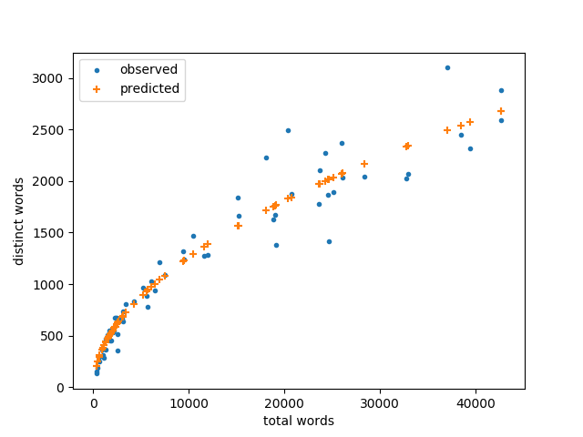
Here’s a visual representation of the results.

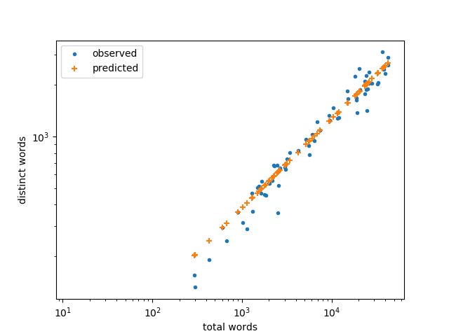
It looks like the predictions are more accurate for small books, and that’s true on an absolute scale. But the relative error is actually smaller for large books as we can see by plotting again on a log-log scale.

Jane Austen novels

It’s a little surprising that Heaps’ law applies well to books of the Bible since the books were composed over centuries and in two different languages. On the other hand, the same committee translated all the books at the same time. Maybe Heaps’ law applies to translations better than it applies to the original texts.

I expect Heaps’ law would fit more closely if you looked at, say, all the novels by a particular author, especially if the author wrote all the books in his or her prime. (I believe I read that someone did a vocabulary analysis of Agatha Christie’s novels and detected a decrease in her vocabulary in her latter years.)

To test this out I looked at Jane Austen’s novels on Project Gutenberg. Here’s the data:

    |-----------------------+--------+------|
    | Novel                 |      n |    V |
    |-----------------------+--------+------|
    | Northanger Abbey      |  78147 | 5995 |
    | Persuasion            |  84117 | 5738 |
    | Sense and Sensibility | 120716 | 6271 |
    | Pride and Prejudice   | 122811 | 6258 |
    | Mansfield Park        | 161454 | 7758 |
    | Emma                  | 161967 | 7092 |
    |-----------------------+--------+------|

The parameters in Heaps’ law work out to K = 121.3 and β = 0.341, a much larger K than before, and a smaller β.

Here’s a comparison of the actual and predicted vocabulary sizes in the novels.

    |-----------------------+------+-------|
    | Novel                 | True | Model |
    |-----------------------+------+-------|
    | Northanger Abbey      | 5995 |  5656 |
    | Persuasion            | 5738 |  5799 |
    | Sense and Sensibility | 6271 |  6560 |
    | Pride and Prejudice   | 6258 |  6598 |
    | Mansfield Park        | 7758 |  7243 |
    | Emma                  | 7092 |  7251 |
    |-----------------------+------+-------|

If a suspected posthumous manuscript of Jane Austen were to appear, a possible test of authenticity would be to look at its vocabulary size to see if it is consistent with her other works. One could also look at the number of words used only once, as we discuss next.

Hapax legomenon

In linguistics, a hapax legomenon is a word that only appears once in a given context. The term comes comes from a Greek phrase meaning something said only once. The term is often shortened to just hapax.

I thought it would be interesting to look at the number of hapax legomena in each book since I could do it with a minor tweak of the code I wrote for the first part of this post.

Normally if someone were speaking of hapax legomena in the context of the Bible, they’d be looking at unique words in the original languages, i.e. Hebrew and Greek, not in English translation. But I’m going with what I have at hand.

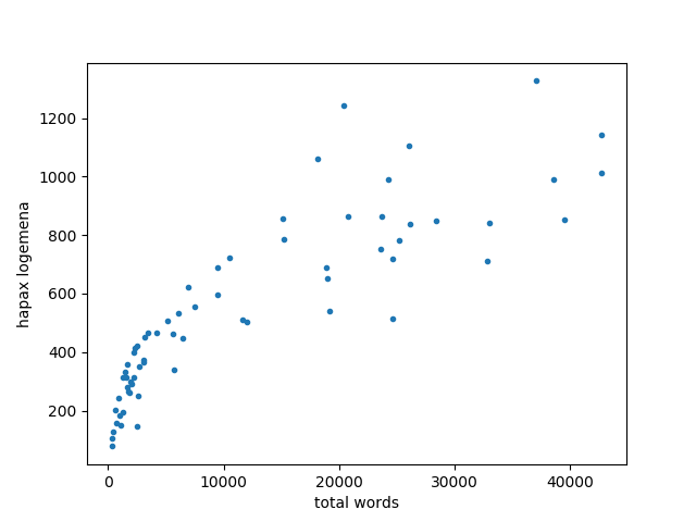
Here’s a plot of the number of haxap in each book of the KJV compared to the number of words in the book.

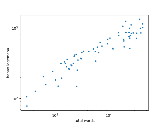
This looks a lot like the plot of vocabulary size and total words, suggesting the number of hapax also follow a power law like Heaps law. This is evident when we plot again on a logarithmic scale and see a linear relation.

Just to be clear on the difference between two analyses this post, in the first we looked at vocabulary size, the number of distinct words in each book. In the second we looked at words that only appear once. In both cases we’re counting unique words, but unique in different senses. In the first analysis, unique means that each word only counts once, no matter how many times it’s used. In the second, unique means that a work only appears once.

Related posts

• Passwords and power laws
• Thou, thee, you, and ye
• Translating poetry

Posted by Adam Gaier, Student Researcher and David Ha, Staff Research Scientist, Google Research, Tokyo

When training a neural network to accomplish a given task, be it image classification or reinforcement learning, one typically refines a set of weights associated with each connection within the network. Another approach to creating successful neural networks that has shown substantial progress is neural architecture search, which constructs neural network architectures out of hand-engineered components such as convolutional network components or transformer blocks. It has been shown that neural network architectures built with these components, such as deep convolutional networks, have strong inductive biases for image processing tasks, and can even perform them when their weights are randomly initialized. While neural architecture search produces new ways of arranging hand-engineered components with known inductive biases for the task domain at hand, there has been little progress in the automated discovery of new neural network architectures with such inductive biases, for various task domains.

We can look at analogies to these useful components in examples of nature vs. nurture. Just as certain precocial species in biology—who possess anti-predator behaviors from the moment of birth—can perform complex motor and sensory tasks without learning, perhaps we can construct network architectures that can perform well without training. Of course, these natural (and by analogy, artificial) neural networks are further improved through training, but their ability to perform even without learning shows that they contain biases that make them well-suited to their task.

In “Weight Agnostic Neural Networks” (WANN), we present a first step toward searching specifically for networks with these biases: neural net architectures that can already perform various tasks, even when they use a random shared weight. Our motivation in this work is to question to what extent neural network architectures alone, without learning any weight parameters, can encode solutions for a given task. By exploring such neural network architectures, we present agents that can already perform well in their environment without the need to learn weight parameters. Furthermore, in order to spur progress in this field community, we have also open-sourced the code to reproduce our WANN experiments for the broader research community.

Left: A hand-engineered, fully-connected deep neural network with 2760 weight connections. Using a learning algorithm, we can solve for the set of 2760 weight parameters so that this network can perform the BipedalWalker-v2 task. Right: A weight agnostic neural network architecture with 44 connections that can perform the same Bipedal Walker task. Unlike the fully-connected network, this WANN can still perform the task without the need to train the weight parameters of each connection. In fact, to simplify the training, the WANN is designed to perform when the values of each weight connection are identical, or shared, and it will even function if this shared weight parameter is randomly sampled.

Finding WANNs
We start with a population of minimal neural network architecture candidates, each with very few connections only, and use a well-established topology search algorithm (NEAT), to evolve the architectures by adding single connections and single nodes one by one. The key idea behind WANNs is to search for architectures by de-emphasizing weights. Unlike traditional neural architecture search methods, where all of the weight parameters of new architectures need to be trained using a learning algorithm, we take a simpler and more efficient approach. Here, during the search, all candidate architectures are first assigned a single shared weight value at each iteration, and then optimized to perform well over a wide range of shared weight values.

Operators for searching the space of network topologies Left: A minimal network topology, with input and outputs only partially connected. Middle: Networks are altered in one of three ways: (1) Insert Node: a new node is inserted by splitting an existing connection. (2) Add Connection: a new connection is added by connecting two previously unconnected nodes. (3) Change Activation: the activation function of a hidden node is reassigned. Right: Possible activation functions (linear, step, sin, cosine, Gaussian, tanh, sigmoid, inverse, absolute value, ReLU)

In addition to exploring a range of weight agnostic neural networks, it is important to also look for network architectures that are only as complex as they need to be. We accomplish this by optimizing for both the performance of the networks and their complexity simultaneously, using techniques drawn from multi-objective optimization.

Overview of Weight Agnostic Neural Network Search and corresponding operators for searching the space of network topologies.

Training WANN Architectures
Unlike traditional networks, we can easily train the WANN by simply finding the best single shared weight parameter that maximizes its performance. In the example below, we see that our architecture works (to some extent) for a swing-up cartpole task using constant weights:

A WANN performing a Cartpole Swing-up task at various different weight parameters, and also using fine-tuned weight parameters.

As we see in the above figure, while WANNs can perform its task using range of shared weight parameters, the performance is still not comparable to a network that learns weights for each individual connection, as normally done in network training. If we want to further improve its performance, we can use the WANN architecture, and the best shared weight as a starting point to fine-tune the weights of each individual connection using a learning algorithm, like how we would normally train any neural network. Using the weight agnostic property of the network architecture as a starting point, and fine-tuning its performance via learning, may help provide insightful analogies to how animals learn.

Through the use of multi-objective optimization for both performance and network simplicity, our method found a simple WANN for a Car Racing from pixels task that works well without explicitly training for the weights of the network.

The ability for a network architecture to function using only random weights offers other advantages too. For instance, by using copies of the same WANN architecture, but where each copy of the WANN is assigned a different distinct weight value, we can create an ensemble of multiple distinct models for the same task. This ensemble generally achieves better performance than a single model. We illustrate this with an example of an MNIST classifier evolved to work with random weights:

An MNIST classifier evolved to work with random weights.

While a conventional network with random initialization will achieve ~10% accuracy on MNIST, this particular network architecture uses random weights and when applied to MNIST achieves an accuracy much better than chance (> 80%). When an ensemble of WANNs is used, each of which assigned with a different shared weight, the accuracy increases to > 90%.

Even without ensemble methods, collapsing the number of weight values in a network to one allows the network to be rapidly tuned. The ability to quickly fine-tune weights might be useful in continual lifelong learning, where agents acquire, adapt, and transfer skills throughout their lifespan. This makes WANNs particularly well positioned to exploit the Baldwin effect, the evolutionary pressure that rewards individuals predisposed to learn useful behaviors, without being trapped in the computationally expensive trap of ‘learning to learn’.

Conclusion
We hope that this work can serve as a stepping stone to help discover novel fundamental neural network components such as the convolutional network, whose discovery and application have been instrumental to the incredible progress made in deep learning. The computational resources available to the research community have grown significantly since the time convolutional neural networks were discovered. If we are devoting such resources to automated discovery and hope to achieve more than incremental improvements in network architectures, we believe it is also worth searching for with new building blocks, not just their arrangements.

If you are interested to learn more about this work, we invite readers to read our interactive article (or pdf version of the paper for offline reading). In addition to open sourcing these experiments to the research community, we have also released a general Python implementation of NEAT called PrettyNEAT to help interested readers to explore the exciting area of neural network evolution from first principles.

Posted by Alex Fabrikant, Research Scientist, Google Research

Hundreds of millions of people across the world rely on public transit for their daily commute, and over half of the world's transit trips involve buses. As the world's cities continue growing, commuters want to know when to expect delays, especially for bus rides, which are prone to getting held up by traffic. While public transit directions provided by Google Maps are informed by many transit agencies that provide real-time data, there are many agencies that can’t provide them due to technical and resource constraints.

Today, Google Maps introduced live traffic delays for buses, forecasting bus delays in hundreds of cities world-wide, ranging from Atlanta to Zagreb to Istanbul to Manila and more. This improves the accuracy of transit timing for over sixty million people. This system, first launched in India three weeks ago, is driven by a machine learning model that combines real-time car traffic forecasts with data on bus routes and stops to better predict how long a bus trip will take.

The Beginnings of a Model
In the many cities without real-time forecasts from the transit agency, we heard from surveyed users that they employed a clever workaround to roughly estimate bus delays: using Google Maps driving directions. But buses are not just large cars. They stop at bus stops; take longer to accelerate, slow down, and turn; and sometimes even have special road privileges, like bus-only lanes.

As an example, let’s examine a Wednesday afternoon bus ride in Sydney. The actual motion of the bus (blue) is running a few minutes behind the published schedule (black). Car traffic speeds (red) do affect the bus, such as the slowdown at 2000 meters, but a long stop at the 800 meter mark slows the bus down significantly compared to a car.
To develop our model, we extracted training data from sequences of bus positions over time, as received from transit agencies’ real time feeds, and aligned them to car traffic speeds on the bus's path during the trip. The model is split into a sequence of timeline units—visits to street blocks and stops—each corresponding to a piece of the bus's timeline, with each unit forecasting a duration. A pair of adjacent observations usually spans many units, due to infrequent reporting, fast-moving buses, and short blocks and stops.

This structure is well suited for neural sequence models like those that have recently been successfully applied to speech processing, machine translation, etc. Our model is simpler. Each unit predicts its duration independently, and the final output is the sum of the per-unit forecasts. Unlike many sequence models, our model does not need to learn to combine unit outputs, nor to pass state through the unit sequence. Instead, the sequence structure lets us jointly (1) train models of individual units' durations and (2) optimize the "linear system" where each observed trajectory assigns a total duration to the sum of the many units it spans.

To model a bus trip (a) starting at the blue stop, the model (b) adds up the delay predictions from timeline units for the blue stop, the three road segments, the white stop, etc.

Modeling the "Where"
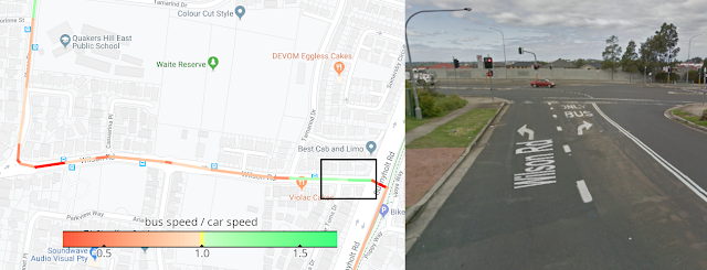
In addition to road traffic delays, in training our model we also take into account details about the bus route, as well as signals about the trip's location and timing. Even within a small neighborhood, the model needs to translate car speed predictions into bus speeds differently on different streets. In the left panel below, we color-code our model's predicted ratio between car speeds and bus speeds for a bus trip. Redder, slower parts may correspond to bus deceleration near stops. As for the fast green stretch in the highlighted box, we learn from looking at it in StreetView (right) that our model discovered a bus-only turn lane. By the way, this route is in Australia, where right turns are slower than left, another aspect that would be lost on a model that doesn’t consider peculiarities of location.
To capture unique properties of specific streets, neighborhoods, and cities, we let the model learn a hierarchy of representations for areas of different size, with a timeline unit's geography (the precise location of a road or a stop) represented in the model by the sum of the embeddings of its location at various scales. We first train the model with progressively heavier penalties for finer-grain locations with special cases, and use the results for feature selection. This ensures that fine-grained features in areas complex enough where a hundred meters affects bus behavior are taken into account, as opposed to open countryside where such fine-grained features seldom matter.

At training time, we also simulate the possibility of later queries about areas that were not in the training data. In each training batch, we take a random slice of examples and discard geographic features below a scale randomly selected for each. Some examples are kept with the exact bus route and street, others keep only neighborhood- or city-level locations, and others yet have no geographical context at all. This better prepares the model for later queries about areas where we were short on training data. We expand the coverage of our training corpus by using anonymized inferences about user bus trips from the same dataset that Google Maps uses for popular times at businesses, parking difficulty, and other features. However, even this data does not include the majority of the world's bus routes, so our models must generalize robustly to new areas.

Learning the Local Rhythms
Different cities and neighborhoods also run to a different beat, so we allow the model to combine its representation of location with time signals. Buses have a complex dependence on time — the difference between 6:30pm and 6:45pm on a Tuesday might be the wind-down of rush hour in some neighborhoods, a busy dining time in others, and entirely quiet in a sleepy town elsewhere. Our model learns an embedding of the local time of day and day of week signals, which, when combined with the location representation, captures salient local variations, like rush hour bus stop crowds, that aren't observed via car traffic.

This embedding assigns 4-dimensional vectors to times of the day. Unlike most neural net internals, four dimensions is almost few enough to visualize, so let's peek at how the model arranges times of day in three of those dimensions, via the artistic rendering below. The model indeed learns that time is cyclical, placing time in a "loop". But this loop is not just the flat circle of a clock's face. The model learns wide bends that let other neurons compose simple rules to easily separate away concepts like "middle of the night" or "late morning" that don't feature much bus behavior variation. On the other hand, evening commute patterns differ much more among neighborhoods and cities, and the model appears to create more complex "crumpled" patterns between 4pm-9pm that enable more intricate inferences about the timings of each city's rush hour.

The model's time representation (3 out of 4 dimensions) forms a loop, reimagined here as the circumference of a watch. The more location-dependent time windows like 4pm-9pm and 7am-9am get more complex "crumpling", while big featureless windows like 2am-5am get bent away with flat bends for simpler rules. (Artist's conception by Will Cassella, using textures from textures.com and HDRIs from hdrihaven.)

Together with other signals, this time representation lets us predict complex patterns even if we hold car speeds constant. On a 10km bus ride through New Jersey, for example, our model picks up on lunchtime crowds and weekday rush hours:
Putting it All Together
With the model fully trained, let's take a look at what it learned about the Sydney bus ride above. If we run the model on that day's car traffic data, it gives us the green predictions below. It doesn't catch everything. For instance, it has the stop at 800 meters lasting only 10 seconds, though the bus stopped for at least 31 sec. But we stay within 1.5 minutes of the real bus motion, catching a lot more of the trip's nuances than the schedule or car driving times alone would give us.
The Trip Ahead
One thing not in our model for now? The bus schedule itself. So far, in experiments with official agency bus schedules, they haven't improved our forecasts significantly. In some cities, severe traffic fluctuations might overwhelm attempts to plan a schedule. In others, the bus schedules might be precise, but perhaps because transit agencies carefully account for traffic patterns. And we infer those from the data.

We continue to experiment with making better use of schedule constraints and many other signals to drive more precise forecasting and make it easier for our users to plan their trips. We hope we'll be of use to you on your way, too. Happy travels!

Acknowledgements
This work was the joint effort of James Cook, Alex Fabrikant, Ivan Kuznetsov, and Fangzhou Xu, on Google Research, and Anthony Bertuca, Julian Gibbons, Thierry Le Boulengé, Cayden Meyer, Anatoli Plotnikov, and Ivan Volosyuk on Google Maps. We thank Senaka Buthpitiya, Da-Cheng Juan, Reuben Kan, Ramesh Nagarajan, Andrew Tomkins, and the greater Transit team for support and helpful discussions; as well as Will Cassella for the inspired reimagining of the model's time embedding. We are also indebted to our partner agencies for providing the transit data feeds the system is trained on.

Posted by Chase Roberts, Research Engineer, Google AI; Stefan Leichenauer, Research Scientist, X

Many of the world's toughest scientific challenges, like developing high-temperature superconductors and understanding the true nature of space and time, involve dealing with the complexity of quantum systems. What makes these challenges difficult is that the number of quantum states in these systems is exponentially large, making brute-force computation infeasible. To deal with this, data structures called tensor networks are used. Tensor networks let one focus on the quantum states that are most relevant for real-world problems—the states of low energy, say—while ignoring other states that aren't relevant. Tensor networks are also increasingly finding applications in machine learning (ML). However, there remain difficulties that prohibit them from widespread use in the ML community: 1) a production-level tensor network library for accelerated hardware has not been available to run tensor network algorithms at scale, and 2) most of the tensor network literature is geared toward physics applications and creates the false impression that expertise in quantum mechanics is required to understand the algorithms.

In order to address these issues, we are releasing TensorNetwork, a brand new open source library to improve the efficiency of tensor calculations, developed in collaboration with the Perimeter Institute for Theoretical Physics and X. TensorNetwork uses TensorFlow as a backend and is optimized for GPU processing, which can enable speedups of up to 100x when compared to work on a CPU. We introduce TensorNetwork in a series of papers, the first of which presents the new library and its API, and provides an overview of tensor networks for a non-physics audience. In our second paper we focus on a particular use case in physics, demonstrating the speedup that one gets using GPUs.

How are Tensor Networks Useful?
Tensors are multidimensional arrays, categorized in a hierarchy according to their order: e.g., an ordinary number is a tensor of order zero (also known as a scalar), a vector is an order-one tensor, a matrix is an order-two tensor, and so on. While low-order tensors can easily be represented by an explicit array of numbers or with a mathematical symbol such as T_ijnklm (where the number of indices represents the order of the tensor), that notation becomes very cumbersome once we start talking about high-order tensors. At that point it’s useful to start using diagrammatic notation, where one simply draws a circle (or some other shape) with a number of lines, or legs, coming out of it—the number of legs being the same as the order of the tensor. In this notation, a scalar is just a circle, a vector has a single leg, a matrix has two legs, etc. Each leg of the tensor also has a dimension, which is the size of that leg. For example, a vector representing an object’s velocity through space would be a three-dimensional, order-one tensor.

Diagrammatic notation for tensors.

The benefit of representing tensors in this way is to succinctly encode mathematical operations, e.g., multiplying a matrix by a vector to produce another vector, or multiplying two vectors to make a scalar. These are all examples of a more general concept called tensor contraction.

Diagrammatic notation for tensor contraction. Vector and matrix multiplication, as well as the matrix trace (i.e., the sum of the diagonal elements of a matrix), are all examples.

These are also simple examples of tensor networks, which are graphical ways of encoding the pattern of tensor contractions of several constituent tensors to form a new one. Each constituent tensor has an order determined by its own number of legs. Legs that are connected, forming an edge in the diagram, represent contraction, while the number of remaining dangling legs determines the order of the resultant tensor.

Left: The trace of the product of four matrices, tr(ABCD), which is a scalar. You can see that it has no dangling legs. Right: Three order-three tensors being contracted with three legs dangling, resulting in a new order-three tensor.

While these examples are very simple, the tensor networks of interest often represent hundreds of tensors contracted in a variety of ways. Describing such a thing would be very obscure using traditional notation, which is why the diagrammatic notation was invented by Roger Penrose in 1971.

Tensor Networks in Practice
Consider a collection of black-and-white images, each of which can be thought of as a list of N pixel values. A single pixel of a single image can be one-hot-encoded into a two-dimensional vector, and by combining these pixel encodings together we can make a 2^N-dimensional one-hot encoding of the entire image. We can reshape that high-dimensional vector into an order-N tensor, and then add up all of the tensors in our collection of images to get a total tensor T_i1,i2,...,iN encapsulating the collection.

This sounds like a very wasteful thing to do: encoding images with about 50 pixels in this way would already take petabytes of memory. That’s where tensor networks come in. Rather than storing or manipulating the tensor T directly, we instead represent T as the contraction of many smaller constituent tensors in the shape of a tensor network. That turns out to be much more efficient. For instance, the popular matrix product state (MPS) network would write T in terms of N much smaller tensors, so that the total number of parameters is only linear in N, rather than exponential.

The high-order tensor T is represented in terms of many low-order tensors in a matrix product state tensor network.

It’s not obvious that large tensor networks can be efficiently created or manipulated while consistently avoiding the need for a huge amount of memory. But it turns out that this is possible in many cases, which is why tensor networks have been used extensively in quantum physics and, now, in machine learning. Stoudenmire and Schwab used the encoding just described to make an image classification model, demonstrating a new use for tensor networks. The TensorNetwork library is designed to facilitate exactly that kind of work, and our first paper describes how the library functions for general tensor network manipulations.

Performance in Physics Use-Cases
TensorNetwork is a general-purpose library for tensor network algorithms, and so it should prove useful for physicists as well. Approximating quantum states is a typical use-case for tensor networks in physics, and is well-suited to illustrate the capabilities of the TensorNetwork library. In our second paper, we describe a tree tensor network (TTN) algorithm for approximating the ground state of either a periodic quantum spin chain (1D) or a lattice model on a thin torus (2D), and implement the algorithm using TensorNetwork. We compare the use of CPUs with GPUs and observe significant computational speed-ups, up to a factor of 100, when using a GPU and the TensorNetwork library.

Computational time as a function of the bond dimension, χ. The bond dimension determines the size of the constituent tensors of the tensor network. A larger bond dimension means the tensor network is more powerful, but requires more computational resources to manipulate.

Conclusion and Future Work
These are the first in a series of planned papers to illustrate the power of TensorNetwork in real-world applications. In our next paper we will use TensorNetwork to classify images in the MNIST and Fashion-MNIST datasets. Future plans include time series analysis on the ML side, and quantum circuit simulation on the physics side. With the open source community, we are also always adding new features to TensorNetwork itself. We hope that TensorNetwork will become a valuable tool for physicists and machine learning practitioners.

Acknowledgements
The TensorNetwork library was developed by Chase Roberts, Adam Zalcman, and Bruce Fontaine of Google AI; Ashley Milsted, Martin Ganahl, and Guifre Vidal of the Perimeter Institute; and Jack Hidary and Stefan Leichenauer of X. We’d also like to thank Stavros Efthymiou at X for valuable contributions.